Solver4J – SDP - semidefinite programming

Consider the problem of minimizing a linear function subject to a matrix inequality as follows:

${minimize}_{x} c^{T} x$   s.t.
     $F (x) \leq 0$
    Ax = b,

with $F (x) = G + \sum_{i = 1}^{m} x_{i} F_{i}$

where $x \in R^{m}$ , $c \in R^{m}$ and $G, F_{1}, ..., F_{m} \in S^{n}$ are $m + 1$ symmetric matrices. The inequality sign in $F (x) \leq 0$ means that $S (x) =-F (x)$ is positive semidefinite, i.e. $v^{T} S (x) v \geq 0$ for all $v \in R^{n}$ . We call the inequality $F (x) \leq 0$ a linear matrix inequality (LMI) and the problem is given the name of semidefinite program (it is a convex optimization problem since its objective and constraints are convex).
See S.Boyd and L.Vandenberghe, "Convex Optimization", p. 168 for a more formal definition and details.

You can use the Barrier Method algorithm available with Solver4J for solving this type of problems, passing in the generalized barrier function for the positive semidefinite cone $S_{+}^{n}$ as the barrier function (see S.Boyd and L.Vandenberghe, "Convex Optimization", p. 600):

$Φ (x) = logdet (- F {(x)}^{- 1})$

with

dom Φ = \{x | F(x) < 0\}

. For strictly feasible x the gradient is equal to

$\frac{dΦ (x)}{{dx}_{i}} = - tr (- F {(x)}^{- 1} F_{i})$

and the hessian is

$\frac{d^{2} Φ (x)}{{dx}_{i} {dx}_{j}} = tr ((- F {(x)}^{- 1} F_{i}) (- F {(x)}^{- 1} F_{j}))$

This function is represented in Solver4J with the class SDPLogarithmicBarrier.

Code example

Here we want to solve a QCQP we already know the solution of as a SDP.
In order to proceed, we first observe (see S.Boyd and L.Vandenberghe, "SEMIDEFINITE PROGRAMMING", SIAM REVIEW Vol. 38, No. 1, pp. 49-95, March 1996) that a convex quadratic constraint

{(Ax + b)}^{T} (Ax + b) - c^{T} x - d \leq 0

, with

x \in R^{k}

, can be written as

$[\begin{matrix} I & Ax + b \\ {(Ax + b)}^{T} & c^{T} x + d \end{matrix}] \geq 0$

The left hand side is an affine function of x, and can be expressed as

$F (x) = G + x_{1} F_{1} + ... + x_{k} F_{k} \leq 0$ with

$G = - [\begin{matrix} I & b \\ b^{T} & d \end{matrix}], F_{i} = - [\begin{matrix} 0 & a_{i} \\ a_{i}^{T} & c_{i} \end{matrix}], i = 1,. .., k$ ( $a_{i}$ are the columns of $A$ )

It follows that a QCQP

${minimize}_{x} f_{0} (x)$ s.t.
$f_{i} (x) \leq 0$ , $i = 1,. .., L$

in which the objective function and the constraints are in the form of:

$f_{i} (x) = {(A_{i} x + b_{i})}^{T} (A_{i} x + b_{i}) - c_{i}^{T} x - d_{i}$ , $i=0,...,L$

can be rewritten as

${minimize}_{x, t} t$   s.t.
     $[\begin{matrix} I & A_{0} x + b_{0} \\ {(A_{0} x + b_{0})}^{T} & c_{0}^{T} x + d_{0} + t \end{matrix}] \geq 0$
     $[\begin{matrix} I & A_{i} x + b_{i} \\ {(A_{i} x + b_{i})}^{T} & c_{i}^{T} x + d_{i} \end{matrix}] \geq 0$ , $i=1,...,L$

which is a SDP with variables

(x, t) \in R^{k + 1}

n = (n_{0} +1) + ... + (n_{L} +1)

and

A_{i} \in R^{n_{i} x k}

, and the matrices G,

F_{i}

are given by

$G = - [\begin{matrix} I & b_{0} & . & . & . & 0 & 0 \\ b_{0}^{T} & d_{0} & 0 & 0 \\ . & . & . \\ . & . & . \\ . & . & . \\ 0 & 0 & I & b_{L} \\ 0 & 0 & . & . & . & b_{L}^{T} & d_{L} \end{matrix}]$

$F_{i} = - [\begin{matrix} 0 & A_{0i} & . & . & . & 0 & 0 \\ A_{0i}^{T} & c_{0} & 0 & 0 \\ . & . & . \\ . & . & . \\ . & . & . \\ 0 & 0 & 0 & A_{Li} \\ 0 & 0 & . & . & . & A_{Li}^{T} & c_{L} \end{matrix}]$ , $i=1,...,k$

.

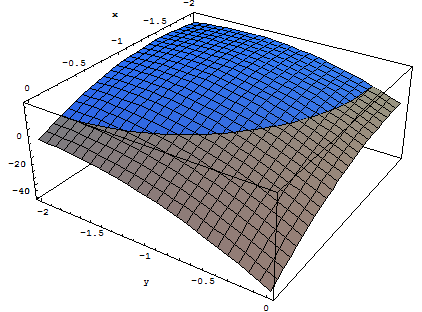
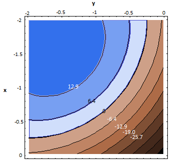
Keeping all this in mind, we now want to find the solution of this QCQP

${minimize}_{x, y} {([\begin{matrix} - \sqrt{\frac{21}{50}} & 0 \\ \frac{- \sqrt{2}}{5} & \frac{- 1}{\sqrt{2}} \end{matrix}] (\begin{matrix} x \\ y \end{matrix}))}^{T} ([\begin{matrix} - \sqrt{\frac{21}{50}} & 0 \\ \frac{- \sqrt{2}}{5} & \frac{- 1}{\sqrt{2}} \end{matrix}] (\begin{matrix} x \\ y \end{matrix}))$ s.t.
${([\begin{matrix} 1 & 0 \\ 0 & 1 \end{matrix}] (\begin{matrix} x \\ y \end{matrix}) + (\begin{matrix} 2 \\ 2 \end{matrix}))}^{T} ([\begin{matrix} 1 & 0 \\ 0 & 1 \end{matrix}] (\begin{matrix} x \\ y \end{matrix}) + (\begin{matrix} 2 \\ 2 \end{matrix})) - {1.75}^{2} \leq 0$

(this is the same problem considered in QCQP - 2D example) threating it as a SDP; for a graphical reference, we show the plot of the function h(x,y)=det(-F(x,y,t)) for a fixed value of t=10 and its level curves in the (x,y) plane: the blue colored surface and curves are relative to the circle that defines the feasible region of the original problem

. It can be do like this:

		
		// Objective function (variables (x,y,t), dim = 3)
		double[] c = new double[]{0,0,1};
		LinearMultivariateRealFunction objectiveFunction = new LinearMultivariateRealFunction(c, 0);
		
		//constraint in the form (A0.x+b0)T.(A0.x+b0) - c0.x - d0 - t < 0
		double[][] A0 = new double[][]{
				{-Math.sqrt(21./50.),  0.             , 0},
				{-Math.sqrt(2)/5.   , -1./Math.sqrt(2), 0}};
		double[] b0 = new double[] { 0, 0, 0 };
		double[] c0 = new double[] { 0, 0, 1 };
		double d0 = 0;
		
		//constraint (this is a circle) in the form (A1.x+b1)T.(A1.x+b1) - c1.x - d1 < 0
		double[][] A1 = new double[][]{{1,0,0},
				                       {0,1,0}};
		double[] b1 = new double[] { 2, 2, 0 };
		double[] c1 = new double[] { 0, 0, 0 };
		double d1 = Math.pow(1.75, 2);
		
		//matrix G for SDP
		double[][] G = new double[][]{
				{1     ,0     ,b0[0] ,0     ,0     ,0},
				{0     ,1     ,b0[1] ,0     ,0     ,0},
				{b0[0] ,b0[1] ,d0    ,0     ,0     ,0},
				{0     ,0     ,0     ,1     ,0     ,b1[0]},
				{0     ,0     ,0     ,0     ,1     ,b1[1]},
				{0     ,0     ,0     ,b1[0] ,b1[1] ,d1}};
		//matrices Fi for SDP
		double[][] F1 =  new double[][]{
				{0        ,0        ,A0[0][0] ,0        ,0        ,0},
				{0        ,0        ,A0[1][0] ,0        ,0        ,0},
				{A0[0][0] ,A0[1][0] ,c0[0]    ,0        ,0        ,0},
				{0        ,0        ,0        ,0        ,0        ,A1[0][0]},
				{0        ,0        ,0        ,0        ,0        ,A1[1][0]},
				{0        ,0        ,0        ,A1[0][0] ,A1[1][0] ,c1[0]}};
		double[][] F2 =  new double[][]{
				{0        ,0        ,A0[0][1] ,0        ,0        ,0},
				{0        ,0        ,A0[1][1] ,0        ,0        ,0},
				{A0[0][1] ,A0[1][1] ,c0[1]    ,0        ,0        ,0},
				{0        ,0        ,0        ,0        ,0        ,A1[0][1]},
				{0        ,0        ,0        ,0        ,0        ,A1[1][1]},
				{0        ,0        ,0        ,A1[0][1] ,A1[1][1] ,c1[1]}};
		double[][] F3 =  new double[][]{
				{0        ,0        ,A0[0][2] ,0        ,0        ,0},
				{0        ,0        ,A0[1][2] ,0        ,0        ,0},
				{A0[0][2] ,A0[1][2] ,c0[2]    ,0        ,0        ,0},
				{0        ,0        ,0        ,0        ,0        ,A1[0][2]},
				{0        ,0        ,0        ,0        ,0        ,A1[1][2]},
				{0        ,0        ,0        ,A1[0][2] ,A1[1][2] ,c1[2]}};
		
		double[][] GMatrix = new Array2DRowRealMatrix(G).scalarMultiply(-1).getData();
		List<double[][]> FiMatrixList = new ArrayList<double[][]>();
		FiMatrixList.add(FiMatrixList.size(), new Array2DRowRealMatrix(F1).scalarMultiply(-1).getData());
		FiMatrixList.add(FiMatrixList.size(), new Array2DRowRealMatrix(F2).scalarMultiply(-1).getData());
		FiMatrixList.add(FiMatrixList.size(), new Array2DRowRealMatrix(F3).scalarMultiply(-1).getData());
		
		//optimization request
		OptimizationRequest or = new OptimizationRequest();
		or.setF0(objectiveFunction);
		//or.setInitialPoint(new double[] { -0.8, -0.8, 10});
		
		//optimization
		BarrierFunction bf = new SDPLogarithmicBarrier(FiMatrixList, GMatrix);
		BarrierMethod opt = new BarrierMethod(bf);
		opt.setOptimizationRequest(or);
		opt.optimize();

This will give the solution:

				double[] sol = opt.getOptimizationResponse().solution;
				sol[0] = -2 + 1.75/Math.sqrt(2)
				sol[1] = -2 + 1.75/Math.sqrt(2)
				sol[2] =  0.8141035444;

Standard form

A SDP is said to be in standard form if it is staded as

${minimize}_{X} tr(CX)$   s.t.
     $tr (A_{i} X) = b_{i}, i=1,...,p$
     $X \geq 0$

with $X \in S^{n}$

see "S.Boyd and L.Vandenberghe, Convex Optimization" example 11.11. Given a problem in standard form, it is simple to formulate and solve it with Solver4J, as shown in the following example.

Code example

		
		//definition of the standard form entities
		int p = 2;
		double[][] C = new double[][]{{2, 1}, {1, 3}};
		double[][] A1 = new double[][]{{2, 1}, {1, 2}};
		double[][] A2 = new double[][]{{5, 2}, {2, 5}};
		double[] b = new double[]{4, 10};
		
		//Solver4J formulation: the variables are the 3 distinctive elements of the symmetric 2x2 matrix X:
		//double[][] X = new double[][]{{x00, x01}, {x01, x11}};
		
		// Objective function: Tr(C, X)
		double[] trCX = new double[]{2, 2, 3};//2*x00 + 2*x01 + 3*x11
		LinearMultivariateRealFunction objectiveFunction = new LinearMultivariateRealFunction(trCX, 0);
		
		// Linear equalities constraints: Tr(A_i, X) = b_i, i=1,2
		double[][] EQcoeff = new double[2][3];
		double[] eqLimits = new double[2];
		EQcoeff[0] = new double[]{2, 2, 2};//2*x00 + 2*x01 + 2*x11 (Tr(A1, X))
		EQcoeff[1] = new double[]{5, 4, 5};//5*x00 + 4*x01 + 5*x11 (Tr(A2, X))
		eqLimits[0] = b[0];
		eqLimits[1] = b[1];
		
		// Linear matrix inequality, i.e X must be semidefinite positive:
		//for this, we decompose X into its components relative to the standard basis of S.
		//The standard basis in the subspace of symmetric matrices S consist of n matrices 
		//that have one element = 1 on the main diagonal (the rest of the elements are 0) and
		//(n-1)+(n-2)+...+2+1 = (n-1)n/2 matrices that have two elements equal 1, the elements 
		//that are placed symmetrically with respect to the main diagonal (remember that
		//symmetric matrices have aij = aji, i!=j)
		double[][] F0 = new double[][]{
				{0 ,0 },
				{0 ,0 }};
		//matrices Fi for SDP: they are the elements of the standard basis of S
		double[][] F1 =  new double[][]{
				{1,0},
				{0,0 }};
		double[][] F2 =  new double[][]{
				{0,1},
				{1,0 }};
		double[][] F3 =  new double[][]{
				{0,0},
				{0,1 }};
		
		double[][] GMatrix = new Array2DRowRealMatrix(F0).scalarMultiply(-1).getData();
		List<double[][]> FiMatrixList = new ArrayList<double[][]>();
		FiMatrixList.add(FiMatrixList.size(), new Array2DRowRealMatrix(F1).scalarMultiply(-1).getData());
		FiMatrixList.add(FiMatrixList.size(), new Array2DRowRealMatrix(F2).scalarMultiply(-1).getData());
		FiMatrixList.add(FiMatrixList.size(), new Array2DRowRealMatrix(F3).scalarMultiply(-1).getData());
		
		//optimization request
		OptimizationRequest or = new OptimizationRequest();
		or.setF0(objectiveFunction);
		or.setInitialPoint(new double[] { 1, 0, 1});
		//or.setNotFeasibleInitialPoint(new double[] { 1, 0, 1});
		or.setCheckKKTSolutionAccuracy(true);
		or.setA(EQcoeff);
		or.setB(eqLimits);
		
		//optimization
		BarrierFunction bf = new SDPLogarithmicBarrier(FiMatrixList, GMatrix);
		BarrierMethod opt = new BarrierMethod(bf);
		opt.setOptimizationRequest(or);
		opt.optimize();

This will give the solution:

					double[] sol = opt.getOptimizationResponse().solution;
					sol[0] = 2;
					sol[1] = 0;
					sol[2] = 0;

Download test source bundle

Download the entire test source bundle from here.