Solver4J – GP - geometric programming

A minimization problem in the form of:

${minimize}_{x} f_{0} (x)$ s.t.
$f_{i} (x) \leq 1, i = 1,. .., m$
$h_{i} (x) = 1, i = 1,...,p$

where $f_{0}, ..., f_{m}$ are posynomials and $h_{0}, ..., h_{p}$ are monomials, and $x \in R_{++}^{n}$ (the constraint $x_{i} > 0$ is implicit)

is called a (standard form) geometric program (GP). See S.Boyd and L.Vandenberghe, "Convex Optimization", 4.5.2 for more details.

We call a function

f : R^{n} \to R

with

dom f = R_{++}^{n}

defined as

$f (x) = {cx}_{1}^{a_{1}} x_{2}^{a_{2}} {⋅⋅⋅x}_{n}^{a_{n}}$

where

c > 0

and

a_{i} \in R

a monomial function or simply a monomial; a sum of monomials, i.e. a function in the form

$f (x) = \sum_{k = 1}^{K} c_{k} x_{1}^{a_{1 k}} x_{2}^{a_{2 k}} {⋅⋅⋅x}_{n}^{a_{n k}}$

where

c_{k} > 0

is called a posynomial function with K terms, or simply a posynomial.

Geometric program are not convex optimization problems, but they can be transformed to convex problems by a change of variables and a transformation of the objective and constraint functions. So, using

$y_{i} = \log (x_{i})$

a posynomial can be rewritten as

$f (x) = \sum_{k = 1}^{K} e^{a_{k}^{T} y + b_{k}}$

where

a_{k} = (a_{1 k}, ..., a_{n k})

and

b_{k} = \log (c_{k})

, and the GP defined above becomes:

${minimize}_{y} \sum_{k = 1}^{K_{0}} e^{a_{0 k}^{T} y + b_{0 k}}$ s.t.
$\sum_{k = 1}^{K_{i}} e^{a_{i k}^{T} y + b_{i k}} \leq 1, i = 1,. .., m$
$e^{g_{i}^{T} y + h_{i}} = 1, i = 1,. .., p$

where

a_{i k} \in R^{n}, i = 0,. .., m

contain the exponents of the posynomial inequality constraints and

g_{i} \in R^{n}, i = 0,. .., p

contain the exponents of the monomial equality constraints of the original geometric program. Now, taking the logarithm of both the objective and constraints functions, we get the problem:

${minimize}_{y} \tilde{f_{0}} (y) = \log (\sum_{k = 1}^{K_{0}} e^{a_{0 k}^{T} y + b_{0 k}})$ s.t.
$\tilde{f_{i}} (y) = \log (\sum_{k = 1}^{K_{i}} e^{a_{i k}^{T} y + b_{i k}}) \leq 0, i = 1,. .., m$
$\tilde{h_{i}} (y) = g_{i}^{T} y + h_{i} = 0, i = 1,. .., p$

This is a convex optimization problem since the functions

\tilde{f_{i}}

are convex and

\tilde{h_{i}}

are affine, and we refer to it as a geometric program in convex form.

2D example

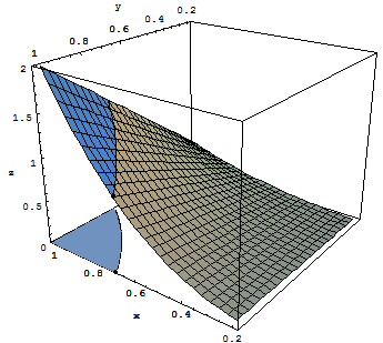
Consider the problem graphically represented hereafter:

that corresponds to:

${minimize}_{(x, y)} x^{2} y + x^{3} y$ s.t.
     $x≤1$
     $y≤1$
     ${0.7x}^{- 1} y^{- 1} \leq 1$

It can be solved like this:

		
		// Objective function (variables (x,y), dim = 2)
		double[] a01 = new double[]{2,1};
		double b01 = 0;
		double[] a02 = new double[]{3,1};
		double b02 = 0;
		ConvexMultivariateRealFunction objectiveFunction = new LogTransformedPosynomial(new double[][]{a01, a02}, new double[]{b01, b02});
		
		//constraints
		double[] a11 = new double[]{1,0};
		double b11 = Math.log(1);
		double[] a21 = new double[]{0,1};
		double b21 = Math.log(1);
		double[] a31 = new double[]{-1,-1.};
		double b31 = Math.log(0.7);
		ConvexMultivariateRealFunction[] inequalities = new ConvexMultivariateRealFunction[3];
		inequalities[0] = new LogTransformedPosynomial(new double[][]{a11}, new double[]{b11});
		inequalities[1] = new LogTransformedPosynomial(new double[][]{a21}, new double[]{b21});
		inequalities[2] = new LogTransformedPosynomial(new double[][]{a31}, new double[]{b31});
		
		//optimization problem
		OptimizationRequest or = new OptimizationRequest();
		or.setF0(objectiveFunction);
		or.setFi(inequalities);
		or.setInitialPoint(new double[]{Math.log(0.9), Math.log(0.9)});
		//or.setInteriorPointMethod(Solver4J.BARRIER_METHOD);//if you prefer the barrier-method
		
		//optimization
		Solver4J opt = new Solver4J();
		opt.setOptimizationRequest(or);
		opt.optimize();

This will give the solution:

				double[] sol = opt.getOptimizationResponse().solution;
				sol[0] = Math.log(0.7);
		    sol[1] = Math.log(1);

and for the original variables it means:

				x = -0.35667494
		    	y =  0.0

Download test source bundle

Download the entire test source bundle from here.